Drawing networks on a plane

Part 4 of a six-part series of adaptations from Terence Tao’s book “Structure and Randomness".

[1.10] The crossing number inequality

A graph $G = (V, E)$ is a set $V$ of vertices ("objects") and a set $E$ of edges ("relationships between two objects"). For example, $V$ could be a set of people and $E$ the set of friendships (Facebook really uses this social graph to analyze user behavior). $V$ could also be the set of airports and $E$ the set of flights from one airport to another. The immense flexibility of this definition allow graphs to model and analyze a tremendous variety of real-life situations, but here we are interested in the abstract representation of a graph, in particular its drawing. The focus is on applying the technique of amplification, which was presented in Part 3 of this series.

A drawing of graph $G = (V, E)$ simply draws the vertices in $V$ as dots on the plane, and the edges $E$ as lines (or curves) connecting them. $G$ can have many possible drawings, in which the edges can have different numbers of crossings between pairs of edges (i.e. three concurrent edges have 3 crossings). Fig. 4(a)-(c) features three drawings of the $K_{3, 3}$ graph with different numbers of crossings.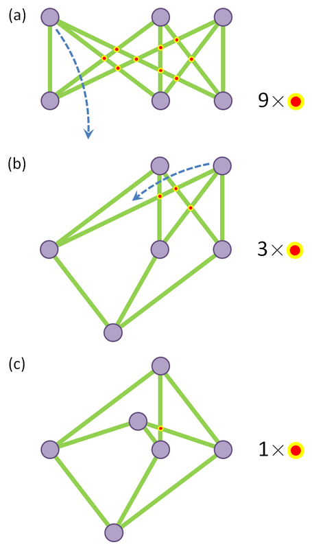

Figure 4: Drawings of K_{3, 3}. Vertices can be moved around to reduce the number of edge crossings (red circles). (a) The usual drawing has 9 crossings. (b) Reduction to 3 crossings. (c) 1 crossing is the minimum.

(Moving vertices to remove crossings is the theme of the wonderful online game Planarity.)

Let $\text{cr}(G)$ denote the minimum number of crossings among all drawings of $G$, also called the crossing number of $G$. The number of vertices $\lvert V\rvert$ is a useful measure of the "size" of $G$; likewise, $\lvert E\rvert$ is a useful measure of the "complexity" of $G$. Thus we attempt to express many quantities related to graphs in terms of these two numbers. For instance, Euler's formula applies when $G$ has a drawing with no crossing edges (i.e. $G$ is planar, and $\text{cr}(G) = 0$):

$$\lvert V\rvert - \lvert E \rvert + \lvert F\rvert = 2 \tag{4.1}$$
where $\lvert F\rvert$ is the number of faces of that non-crossing drawing, i.e. the number of regions the plane is divided into by the edges (verify it for a drawing of a chessboard!). You may recall this formula as the Euler characteristic for polyhedra; the analogy is obvious when you think of stretching a polyhedron open and squashing it into the plane, drawing a planar graph.

We'd like to relate $\text{cr}(G)$ to $\lvert V\rvert$ and $\lvert E\rvert$, but two graphs can have the same number of vertices and edges yet different crossing numbers (find two such graphs!). The next best thing is a bound in terms of $\lvert V\rvert$ and $\lvert E\rvert$, one of which we derive here—the crossing number inequality:

$$\text{cr}(G) \geq \lvert E\rvert^3/(64\lvert V\rvert^2) \text{ whenever } \lvert E\rvert \geq 4\lvert V\rvert \tag{4.2}$$
The condition $\lvert E \rvert \geq 4\lvert V \rvert$ requires that $G$ is "complex enough" relative to its size; this bound is useful because we are mainly interested in the behavior of complicated graphs.

Unbelievably, this bound is the result of amplifying (twice) an inequality that is rather trivial in comparison; this "starting point" is the relationship between $\lvert V\rvert$ and $\lvert E\rvert$ when $G$ is planar. Since each edge touches 2 faces and each face touches at least 3 edges, we have the "starting point" $3\lvert F\rvert \leq 2\lvert E\rvert$ (when does equality hold?). Substituting into Eq. (4.1), we have
$$\lvert E\rvert \leq 3\lvert V\rvert - 6 \text{ whenever } \text{cr}(G) = 0 \tag{4.3}$$
We now amplify by exploiting the symmetry due to the "freedom to look at a subgraph" (a smaller graph obtained by deleting some edges or vertices), something like self-similarity. The crucial observations are:

• An imbalance in this symmetry occurs if we remove edges from $G$, because the RHS of Eq. (4.3) is unaffected.
• Removing edges can remove crossings.

Suppose that $\text{cr}(G) > 0$. Find the drawing of $G$ with that number of crossings. For each crossing, remove one of the edges involved; this eliminates all of the crossings by removing at most $\text{cr}(G)$ edges. With no more crossings left, we apply Eq. (4.3) to this smaller graph to get

$$\lvert E\rvert - \text{cr}(G) \leq 3\lvert V\rvert - 6 \implies \text{cr}(G) \geq \lvert E\rvert - 3\lvert V\rvert + 6. \tag{4.4}$$
Eq. (4.4) is our first "real" bound. We amplify more, this time by removing vertices (and the edges touching them). This indirectly removes crossings, but for the sake of a strong bound we want to remove many crossings with few vertices. Which vertices should we choose? We call upon the counter-intuitive probabilistic method from combinatorics:

... if there is no obvious "best" choice for some combinatorial object (such as a set of vertices to delete), then trying a random choice will often give a reasonable answer, provided the notion of "random" is chosen carefully.

[1.10, p. 97]

Hence we randomly remove each vertex with a probability $(1 - p)$. Vertices survive with probability $p$, edges with probability $p^2$ (both endpoints must survive), and crossings with probability less than $p^4$ (see the full reasoning). We apply Eq. (4.4) to the "expected surviving graph" to obtain

$$p^4\text{cr}(G) \geq p^2\lvert E\rvert - 3p\lvert V\rvert + 6 \implies \text{cr}(G) \geq p^{-2}\lvert E\rvert - 3p^{-3}\lvert V\rvert + 6p^{-4} \tag{4.5}$$
The crossing number inequality (Eq. (4.2)) results from increasing the RHS of Eq. (4.5) by tweaking the value of $p$.

Further discussion

My explanation of how the probabilistic method is used here risks oversimplification; I urge readers to look up the full argument in the original blog post.

The crossing number inequality is very strong and, as a result, very useful (see "Why do we need strong inequalities?" in Part 3 of this series). The original blog post lists two of its applications, including an easy derivation of the Szemerédi-Trotter theorem, which bounds the number of point-line incidences that can occur given a collection of points and lines on a plane. The connection arises by viewing the setup as the drawing of a graph: points are vertices, and lines containing many points can be broken into edges connecting those points.

References

[1.10] Tao, Terence. The crossing number inequality. In Structure and Randomness: Pages from Year One of a Mathematical Blog. American Mathematical Society (2008).